03 Regression (Exercise 15)
Yeon Soo, Choi
15. Boston Data
Boston 데이터는 crim, zn, indus, chas, nox, rm, age, dis, rad, tax, ptratio, black, lstat, medv 이렇게 14개의 변수들로 이루어져 있으며,
15번 예제의 경우 마을 별 인당 범죄율 에 대한 정보를 갖는 crim 변수를 종속변수 로 사용하여 예측하는 것이 목표다.
library(knitr)
library(MASS)
data(Boston)
str(Boston)
## 'data.frame':    506 obs. of  14 variables:
##  $ crim   : num  0.00632 0.02731 0.02729 0.03237 0.06905 ...
##  $ zn     : num  18 0 0 0 0 0 12.5 12.5 12.5 12.5 ...
##  $ indus  : num  2.31 7.07 7.07 2.18 2.18 2.18 7.87 7.87 7.87 7.87 ...
##  $ chas   : int  0 0 0 0 0 0 0 0 0 0 ...
##  $ nox    : num  0.538 0.469 0.469 0.458 0.458 0.458 0.524 0.524 0.524 0.524 ...
##  $ rm     : num  6.58 6.42 7.18 7 7.15 ...
##  $ age    : num  65.2 78.9 61.1 45.8 54.2 58.7 66.6 96.1 100 85.9 ...
##  $ dis    : num  4.09 4.97 4.97 6.06 6.06 ...
##  $ rad    : int  1 2 2 3 3 3 5 5 5 5 ...
##  $ tax    : num  296 242 242 222 222 222 311 311 311 311 ...
##  $ ptratio: num  15.3 17.8 17.8 18.7 18.7 18.7 15.2 15.2 15.2 15.2 ...
##  $ black  : num  397 397 393 395 397 ...
##  $ lstat  : num  4.98 9.14 4.03 2.94 5.33 ...
##  $ medv   : num  24 21.6 34.7 33.4 36.2 28.7 22.9 27.1 16.5 18.9 ...
colSums(is.na(Boston))
##    crim      zn   indus    chas     nox      rm     age     dis     rad
##       0       0       0       0       0       0       0       0       0
##     tax ptratio   black   lstat    medv
##       0       0       0       0       0
## chas : Charles River dummy variable (=1 bounds river, =0 otherwise)
Boston$chas=factor(Boston$chas,c(0,1),labels=c('N','Y'))
kable(head(Boston))
| crim | zn | indus | chas | nox | rm | age | dis | rad | tax | ptratio | black | lstat | medv |
|---|---|---|---|---|---|---|---|---|---|---|---|---|---|
| 0.00632 | 18 | 2.31 | N | 0.538 | 6.575 | 65.2 | 4.0900 | 1 | 296 | 15.3 | 396.90 | 4.98 | 24.0 |
| 0.02731 | 0 | 7.07 | N | 0.469 | 6.421 | 78.9 | 4.9671 | 2 | 242 | 17.8 | 396.90 | 9.14 | 21.6 |
| 0.02729 | 0 | 7.07 | N | 0.469 | 7.185 | 61.1 | 4.9671 | 2 | 242 | 17.8 | 392.83 | 4.03 | 34.7 |
| 0.03237 | 0 | 2.18 | N | 0.458 | 6.998 | 45.8 | 6.0622 | 3 | 222 | 18.7 | 394.63 | 2.94 | 33.4 |
| 0.06905 | 0 | 2.18 | N | 0.458 | 7.147 | 54.2 | 6.0622 | 3 | 222 | 18.7 | 396.90 | 5.33 | 36.2 |
| 0.02985 | 0 | 2.18 | N | 0.458 | 6.430 | 58.7 | 6.0622 | 3 | 222 | 18.7 | 394.12 | 5.21 | 28.7 |
(a) 각각의 독립 변수들로 단순 선형 회귀 모형을 적합하고 통계적으로 유의한 모형인지 아닌지 판단하여라.
library(caret)
## Loading required package: lattice

## Loading required package: ggplot2
library(corrplot)
## corrplot 0.84 loaded
preds=names(Boston)[c(2:3,5:14)]
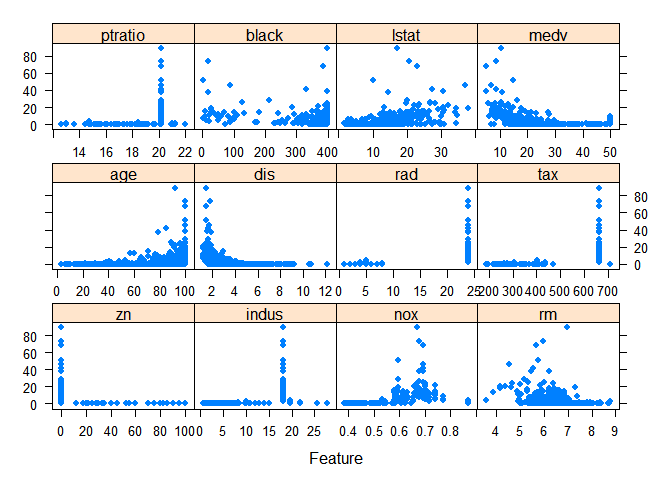
## plot response by predictors
featurePlot(x=Boston[,preds],y=Boston$crim,pch=20,cex=1.2)

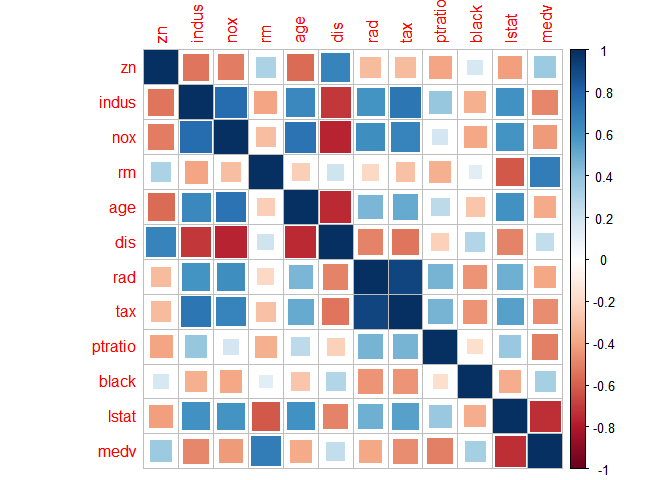
corrplot(cor(Boston[,preds]),method='square')
ZN : proportion of residential land zoned for lots over 25,000 sq.ft.
## 13 simple linear regression models
attach(Boston)
## yes
lm.zn = lm(crim~zn)
summary(lm.zn)
##
## Call:
## lm(formula = crim ~ zn)
##
## Residuals:
##    Min     1Q Median     3Q    Max
## -4.429 -4.222 -2.620  1.250 84.523
##
## Coefficients:
##             Estimate Std. Error t value Pr(>|t|)
## (Intercept)  4.45369    0.41722  10.675  < 2e-16 ***
## zn          -0.07393    0.01609  -4.594 5.51e-06 ***
## ---
## Signif. codes:  0 '***' 0.001 '**' 0.01 '*' 0.05 '.' 0.1 ' ' 1
##
## Residual standard error: 8.435 on 504 degrees of freedom
## Multiple R-squared:  0.04019,    Adjusted R-squared:  0.03828
## F-statistic:  21.1 on 1 and 504 DF,  p-value: 5.506e-06
INDUS : proportion of non-retail business acres per town.
## yes
lm.indus = lm(crim~indus)
summary(lm.indus)
##
## Call:
## lm(formula = crim ~ indus)
##
## Residuals:
##     Min      1Q  Median      3Q     Max
## -11.972  -2.698  -0.736   0.712  81.813
##
## Coefficients:
##             Estimate Std. Error t value Pr(>|t|)
## (Intercept) -2.06374    0.66723  -3.093  0.00209 **
## indus        0.50978    0.05102   9.991  < 2e-16 ***
## ---
## Signif. codes:  0 '***' 0.001 '**' 0.01 '*' 0.05 '.' 0.1 ' ' 1
##
## Residual standard error: 7.866 on 504 degrees of freedom
## Multiple R-squared:  0.1653, Adjusted R-squared:  0.1637
## F-statistic: 99.82 on 1 and 504 DF,  p-value: < 2.2e-16
CHAS : Charles River dummy variable (= 1 if tract bounds river; 0 otherwise).
## no
lm.chas = lm(crim~chas)
summary(lm.chas)
##
## Call:
## lm(formula = crim ~ chas)
##
## Residuals:
##    Min     1Q Median     3Q    Max
## -3.738 -3.661 -3.435  0.018 85.232
##
## Coefficients:
##             Estimate Std. Error t value Pr(>|t|)
## (Intercept)   3.7444     0.3961   9.453   <2e-16 ***
## chasY        -1.8928     1.5061  -1.257    0.209
## ---
## Signif. codes:  0 '***' 0.001 '**' 0.01 '*' 0.05 '.' 0.1 ' ' 1
##
## Residual standard error: 8.597 on 504 degrees of freedom
## Multiple R-squared:  0.003124,   Adjusted R-squared:  0.001146
## F-statistic: 1.579 on 1 and 504 DF,  p-value: 0.2094
NOX : nitrogen oxides concentration (parts per 10 million).
## yes
lm.nox = lm(crim~nox)
summary(lm.nox)
##
## Call:
## lm(formula = crim ~ nox)
##
## Residuals:
##     Min      1Q  Median      3Q     Max
## -12.371  -2.738  -0.974   0.559  81.728
##
## Coefficients:
##             Estimate Std. Error t value Pr(>|t|)
## (Intercept)  -13.720      1.699  -8.073 5.08e-15 ***
## nox           31.249      2.999  10.419  < 2e-16 ***
## ---
## Signif. codes:  0 '***' 0.001 '**' 0.01 '*' 0.05 '.' 0.1 ' ' 1
##
## Residual standard error: 7.81 on 504 degrees of freedom
## Multiple R-squared:  0.1772, Adjusted R-squared:  0.1756
## F-statistic: 108.6 on 1 and 504 DF,  p-value: < 2.2e-16
RM : average number of rooms per dwelling.
## yes
lm.rm = lm(crim~rm)
summary(lm.rm)
##
## Call:
## lm(formula = crim ~ rm)
##
## Residuals:
##    Min     1Q Median     3Q    Max
## -6.604 -3.952 -2.654  0.989 87.197
##
## Coefficients:
##             Estimate Std. Error t value Pr(>|t|)
## (Intercept)   20.482      3.365   6.088 2.27e-09 ***
## rm            -2.684      0.532  -5.045 6.35e-07 ***
## ---
## Signif. codes:  0 '***' 0.001 '**' 0.01 '*' 0.05 '.' 0.1 ' ' 1
##
## Residual standard error: 8.401 on 504 degrees of freedom
## Multiple R-squared:  0.04807,    Adjusted R-squared:  0.04618
## F-statistic: 25.45 on 1 and 504 DF,  p-value: 6.347e-07
AGE : proportion of owner-occupied units built prior to 1940.
## yes
lm.age = lm(crim~age)
summary(lm.age)
##
## Call:
## lm(formula = crim ~ age)
##
## Residuals:
##    Min     1Q Median     3Q    Max
## -6.789 -4.257 -1.230  1.527 82.849
##
## Coefficients:
##             Estimate Std. Error t value Pr(>|t|)
## (Intercept) -3.77791    0.94398  -4.002 7.22e-05 ***
## age          0.10779    0.01274   8.463 2.85e-16 ***
## ---
## Signif. codes:  0 '***' 0.001 '**' 0.01 '*' 0.05 '.' 0.1 ' ' 1
##
## Residual standard error: 8.057 on 504 degrees of freedom
## Multiple R-squared:  0.1244, Adjusted R-squared:  0.1227
## F-statistic: 71.62 on 1 and 504 DF,  p-value: 2.855e-16
DIS : weighted mean of distances to five Boston employment centres.
## yes
lm.dis = lm(crim~dis)
summary(lm.dis)
##
## Call:
## lm(formula = crim ~ dis)
##
## Residuals:
##    Min     1Q Median     3Q    Max
## -6.708 -4.134 -1.527  1.516 81.674
##
## Coefficients:
##             Estimate Std. Error t value Pr(>|t|)
## (Intercept)   9.4993     0.7304  13.006   <2e-16 ***
## dis          -1.5509     0.1683  -9.213   <2e-16 ***
## ---
## Signif. codes:  0 '***' 0.001 '**' 0.01 '*' 0.05 '.' 0.1 ' ' 1
##
## Residual standard error: 7.965 on 504 degrees of freedom
## Multiple R-squared:  0.1441, Adjusted R-squared:  0.1425
## F-statistic: 84.89 on 1 and 504 DF,  p-value: < 2.2e-16
RAD : index of accessibility to radial highways.
## yes
lm.rad = lm(crim~rad)
summary(lm.rad)
##
## Call:
## lm(formula = crim ~ rad)
##
## Residuals:
##     Min      1Q  Median      3Q     Max
## -10.164  -1.381  -0.141   0.660  76.433
##
## Coefficients:
##             Estimate Std. Error t value Pr(>|t|)
## (Intercept) -2.28716    0.44348  -5.157 3.61e-07 ***
## rad          0.61791    0.03433  17.998  < 2e-16 ***
## ---
## Signif. codes:  0 '***' 0.001 '**' 0.01 '*' 0.05 '.' 0.1 ' ' 1
##
## Residual standard error: 6.718 on 504 degrees of freedom
## Multiple R-squared:  0.3913, Adjusted R-squared:   0.39
## F-statistic: 323.9 on 1 and 504 DF,  p-value: < 2.2e-16
TAX : full-value property-tax rate per $10,000.
## yes
lm.tax = lm(crim~tax)
summary(lm.tax)
##
## Call:
## lm(formula = crim ~ tax)
##
## Residuals:
##     Min      1Q  Median      3Q     Max
## -12.513  -2.738  -0.194   1.065  77.696
##
## Coefficients:
##              Estimate Std. Error t value Pr(>|t|)
## (Intercept) -8.528369   0.815809  -10.45   <2e-16 ***
## tax          0.029742   0.001847   16.10   <2e-16 ***
## ---
## Signif. codes:  0 '***' 0.001 '**' 0.01 '*' 0.05 '.' 0.1 ' ' 1
##
## Residual standard error: 6.997 on 504 degrees of freedom
## Multiple R-squared:  0.3396, Adjusted R-squared:  0.3383
## F-statistic: 259.2 on 1 and 504 DF,  p-value: < 2.2e-16
PTRATIO : pupil-teacher ratio by town.
## yes
lm.ptratio = lm(crim~ptratio)
summary(lm.ptratio)
##
## Call:
## lm(formula = crim ~ ptratio)
##
## Residuals:
##    Min     1Q Median     3Q    Max
## -7.654 -3.985 -1.912  1.825 83.353
##
## Coefficients:
##             Estimate Std. Error t value Pr(>|t|)
## (Intercept) -17.6469     3.1473  -5.607 3.40e-08 ***
## ptratio       1.1520     0.1694   6.801 2.94e-11 ***
## ---
## Signif. codes:  0 '***' 0.001 '**' 0.01 '*' 0.05 '.' 0.1 ' ' 1
##
## Residual standard error: 8.24 on 504 degrees of freedom
## Multiple R-squared:  0.08407,    Adjusted R-squared:  0.08225
## F-statistic: 46.26 on 1 and 504 DF,  p-value: 2.943e-11
BLACK : 1000(Bk - 0.63)^2 where Bk is the proportion of blacks by town.
## yes
lm.black = lm(crim~black)
summary(lm.black)
##
## Call:
## lm(formula = crim ~ black)
##
## Residuals:
##     Min      1Q  Median      3Q     Max
## -13.756  -2.299  -2.095  -1.296  86.822
##
## Coefficients:
##              Estimate Std. Error t value Pr(>|t|)
## (Intercept) 16.553529   1.425903  11.609   <2e-16 ***
## black       -0.036280   0.003873  -9.367   <2e-16 ***
## ---
## Signif. codes:  0 '***' 0.001 '**' 0.01 '*' 0.05 '.' 0.1 ' ' 1
##
## Residual standard error: 7.946 on 504 degrees of freedom
## Multiple R-squared:  0.1483, Adjusted R-squared:  0.1466
## F-statistic: 87.74 on 1 and 504 DF,  p-value: < 2.2e-16
LSTAT : lower status of the population (percent).
## yes
lm.lstat = lm(crim~lstat)
summary(lm.lstat)
##
## Call:
## lm(formula = crim ~ lstat)
##
## Residuals:
##     Min      1Q  Median      3Q     Max
## -13.925  -2.822  -0.664   1.079  82.862
##
## Coefficients:
##             Estimate Std. Error t value Pr(>|t|)
## (Intercept) -3.33054    0.69376  -4.801 2.09e-06 ***
## lstat        0.54880    0.04776  11.491  < 2e-16 ***
## ---
## Signif. codes:  0 '***' 0.001 '**' 0.01 '*' 0.05 '.' 0.1 ' ' 1
##
## Residual standard error: 7.664 on 504 degrees of freedom
## Multiple R-squared:  0.2076, Adjusted R-squared:  0.206
## F-statistic:   132 on 1 and 504 DF,  p-value: < 2.2e-16
MEDV : median value of owner-occupied homes in $1000s.
lm.medv = lm(crim~medv)
summary(lm.medv)
##
## Call:
## lm(formula = crim ~ medv)
##
## Residuals:
##    Min     1Q Median     3Q    Max
## -9.071 -4.022 -2.343  1.298 80.957
##
## Coefficients:
##             Estimate Std. Error t value Pr(>|t|)
## (Intercept) 11.79654    0.93419   12.63   <2e-16 ***
## medv        -0.36316    0.03839   -9.46   <2e-16 ***
## ---
## Signif. codes:  0 '***' 0.001 '**' 0.01 '*' 0.05 '.' 0.1 ' ' 1
##
## Residual standard error: 7.934 on 504 degrees of freedom
## Multiple R-squared:  0.1508, Adjusted R-squared:  0.1491
## F-statistic: 89.49 on 1 and 504 DF,  p-value: < 2.2e-16
chas 변수를 제외하고 모두 계수의 유의성 검정 결과 유의하다고 결론지었다.
(b) 모든 독립변수들을 사용하여 다중 선형 회귀 모형을 적합하여라. 결과를 설명하고 어떤 독립변수들이 T-검정 하의 단일 계수의 유의성 검정 결과 유의한가?
95% 신뢰 수준에서 T-검정으로 계수의 유의성에 대해 검정한 결과 zn, dis, rad, black, medv 다섯 가지 변수들이 통계적으로 유의하다고 결론지었다.
lm.all = lm(crim~., data=Boston)
summary(lm.all)
##
## Call:
## lm(formula = crim ~ ., data = Boston)
##
## Residuals:
##    Min     1Q Median     3Q    Max
## -9.924 -2.120 -0.353  1.019 75.051
##
## Coefficients:
##               Estimate Std. Error t value Pr(>|t|)
## (Intercept)  17.033228   7.234903   2.354 0.018949 *
## zn            0.044855   0.018734   2.394 0.017025 *
## indus        -0.063855   0.083407  -0.766 0.444294
## chasY        -0.749134   1.180147  -0.635 0.525867
## nox         -10.313535   5.275536  -1.955 0.051152 .
## rm            0.430131   0.612830   0.702 0.483089
## age           0.001452   0.017925   0.081 0.935488
## dis          -0.987176   0.281817  -3.503 0.000502 ***
## rad           0.588209   0.088049   6.680 6.46e-11 ***
## tax          -0.003780   0.005156  -0.733 0.463793
## ptratio      -0.271081   0.186450  -1.454 0.146611
## black        -0.007538   0.003673  -2.052 0.040702 *
## lstat         0.126211   0.075725   1.667 0.096208 .
## medv         -0.198887   0.060516  -3.287 0.001087 **
## ---
## Signif. codes:  0 '***' 0.001 '**' 0.01 '*' 0.05 '.' 0.1 ' ' 1
##
## Residual standard error: 6.439 on 492 degrees of freedom
## Multiple R-squared:  0.454,  Adjusted R-squared:  0.4396
## F-statistic: 31.47 on 13 and 492 DF,  p-value: < 2.2e-16
(c) 단순선형회귀에서의 계수 값들을 X축에, 다중선형회귀에서의 계수 값들을 Y축에 그려내 비교하여라.
x = c(coefficients(lm.zn)[2],
      coefficients(lm.indus)[2],
      coefficients(lm.chas)[2],
      coefficients(lm.nox)[2],
      coefficients(lm.rm)[2],
      coefficients(lm.age)[2],
      coefficients(lm.dis)[2],
      coefficients(lm.rad)[2],
      coefficients(lm.tax)[2],
      coefficients(lm.ptratio)[2],
      coefficients(lm.black)[2],
      coefficients(lm.lstat)[2],
      coefficients(lm.medv)[2])
y = coefficients(lm.all)[2:14]
z = names(Boston)[2:14]
c=data.frame(x=x,y=y,z=z)

library(ggplot2)

ggplot(c)+
  geom_point(aes(x=x,y=y,color=z),size=2)+
  theme_classic()+
  xlab('Simple Linear Regression Coefficient Estimates')+
  ylab('Multiple Linear Regression Coefficient Estimates')+
  ggtitle('Comparison of Coefficient Estimates')
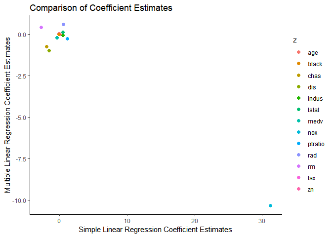
nox 변수의 경우 단순 선형 회귀 모형에서의 계수가 약 31 이었던 반면 다중선형회귀에서는 약 -10 의 값을 갖는 눈에 띄는 차이가 발견되었다.
(d) 독립변수와 종속변수 간의 비선형 관계가 존재한다는 증거가 있는가? 이를 확인하기 위해 3차 다항 회귀를 적합하여라.
앞서 그렸던 종속변수 crim 에 대해 각각의 독립변수를 그려낸 결과를 통해서도 비선형 관계가 존재한다는 것을 알 수 있다.
featurePlot(x=Boston[,preds],y=Boston$crim,pch=20,cex=1.2)
우선 문제에서 주어진 대로 3차 다항회귀를 적합한 결과는 다음과 같다.
zn3=lm(crim~poly(zn,3),Boston)
indus3=lm(crim~poly(indus,3),Boston)
nox3=lm(crim~poly(nox,3),Boston)
rm3=lm(crim~poly(rm,3),Boston)
age3=lm(crim~poly(age,3),Boston)
dis3=lm(crim~poly(dis,3),Boston)
rad3=lm(crim~poly(rad,3),Boston)
tax3=lm(crim~poly(tax,3),Boston)
ptratio3=lm(crim~poly(ptratio,3),Boston)
black3=lm(crim~poly(black,3),Boston)
lstat3=lm(crim~poly(lstat,3),Boston)
medv3=lm(crim~poly(medv,3),Boston)
ZN
## 1,2
summary(zn3)
##
## Call:
## lm(formula = crim ~ poly(zn, 3), data = Boston)
##
## Residuals:
##    Min     1Q Median     3Q    Max
## -4.821 -4.614 -1.294  0.473 84.130
##
## Coefficients:
##              Estimate Std. Error t value Pr(>|t|)
## (Intercept)    3.6135     0.3722   9.709  < 2e-16 ***
## poly(zn, 3)1 -38.7498     8.3722  -4.628  4.7e-06 ***
## poly(zn, 3)2  23.9398     8.3722   2.859  0.00442 **
## poly(zn, 3)3 -10.0719     8.3722  -1.203  0.22954
## ---
## Signif. codes:  0 '***' 0.001 '**' 0.01 '*' 0.05 '.' 0.1 ' ' 1
##
## Residual standard error: 8.372 on 502 degrees of freedom
## Multiple R-squared:  0.05824,    Adjusted R-squared:  0.05261
## F-statistic: 10.35 on 3 and 502 DF,  p-value: 1.281e-06
INDUS
## 1,2,3
summary(indus3)
##
## Call:
## lm(formula = crim ~ poly(indus, 3), data = Boston)
##
## Residuals:
##    Min     1Q Median     3Q    Max
## -8.278 -2.514  0.054  0.764 79.713
##
## Coefficients:
##                 Estimate Std. Error t value Pr(>|t|)
## (Intercept)        3.614      0.330  10.950  < 2e-16 ***
## poly(indus, 3)1   78.591      7.423  10.587  < 2e-16 ***
## poly(indus, 3)2  -24.395      7.423  -3.286  0.00109 **
## poly(indus, 3)3  -54.130      7.423  -7.292  1.2e-12 ***
## ---
## Signif. codes:  0 '***' 0.001 '**' 0.01 '*' 0.05 '.' 0.1 ' ' 1
##
## Residual standard error: 7.423 on 502 degrees of freedom
## Multiple R-squared:  0.2597, Adjusted R-squared:  0.2552
## F-statistic: 58.69 on 3 and 502 DF,  p-value: < 2.2e-16
NOX
## 1,2,3
summary(nox3)
##
## Call:
## lm(formula = crim ~ poly(nox, 3), data = Boston)
##
## Residuals:
##    Min     1Q Median     3Q    Max
## -9.110 -2.068 -0.255  0.739 78.302
##
## Coefficients:
##               Estimate Std. Error t value Pr(>|t|)
## (Intercept)     3.6135     0.3216  11.237  < 2e-16 ***
## poly(nox, 3)1  81.3720     7.2336  11.249  < 2e-16 ***
## poly(nox, 3)2 -28.8286     7.2336  -3.985 7.74e-05 ***
## poly(nox, 3)3 -60.3619     7.2336  -8.345 6.96e-16 ***
## ---
## Signif. codes:  0 '***' 0.001 '**' 0.01 '*' 0.05 '.' 0.1 ' ' 1
##
## Residual standard error: 7.234 on 502 degrees of freedom
## Multiple R-squared:  0.297,  Adjusted R-squared:  0.2928
## F-statistic: 70.69 on 3 and 502 DF,  p-value: < 2.2e-16
RM
## 1,2
summary(rm3)
##
## Call:
## lm(formula = crim ~ poly(rm, 3), data = Boston)
##
## Residuals:
##     Min      1Q  Median      3Q     Max
## -18.485  -3.468  -2.221  -0.015  87.219
##
## Coefficients:
##              Estimate Std. Error t value Pr(>|t|)
## (Intercept)    3.6135     0.3703   9.758  < 2e-16 ***
## poly(rm, 3)1 -42.3794     8.3297  -5.088 5.13e-07 ***
## poly(rm, 3)2  26.5768     8.3297   3.191  0.00151 **
## poly(rm, 3)3  -5.5103     8.3297  -0.662  0.50858
## ---
## Signif. codes:  0 '***' 0.001 '**' 0.01 '*' 0.05 '.' 0.1 ' ' 1
##
## Residual standard error: 8.33 on 502 degrees of freedom
## Multiple R-squared:  0.06779,    Adjusted R-squared:  0.06222
## F-statistic: 12.17 on 3 and 502 DF,  p-value: 1.067e-07
AGE
## 1,2,3
summary(age3)
##
## Call:
## lm(formula = crim ~ poly(age, 3), data = Boston)
##
## Residuals:
##    Min     1Q Median     3Q    Max
## -9.762 -2.673 -0.516  0.019 82.842
##
## Coefficients:
##               Estimate Std. Error t value Pr(>|t|)
## (Intercept)     3.6135     0.3485  10.368  < 2e-16 ***
## poly(age, 3)1  68.1820     7.8397   8.697  < 2e-16 ***
## poly(age, 3)2  37.4845     7.8397   4.781 2.29e-06 ***
## poly(age, 3)3  21.3532     7.8397   2.724  0.00668 **
## ---
## Signif. codes:  0 '***' 0.001 '**' 0.01 '*' 0.05 '.' 0.1 ' ' 1
##
## Residual standard error: 7.84 on 502 degrees of freedom
## Multiple R-squared:  0.1742, Adjusted R-squared:  0.1693
## F-statistic: 35.31 on 3 and 502 DF,  p-value: < 2.2e-16
DIS
## 1,2,3
summary(dis3)
##
## Call:
## lm(formula = crim ~ poly(dis, 3), data = Boston)
##
## Residuals:
##     Min      1Q  Median      3Q     Max
## -10.757  -2.588   0.031   1.267  76.378
##
## Coefficients:
##               Estimate Std. Error t value Pr(>|t|)
## (Intercept)     3.6135     0.3259  11.087  < 2e-16 ***
## poly(dis, 3)1 -73.3886     7.3315 -10.010  < 2e-16 ***
## poly(dis, 3)2  56.3730     7.3315   7.689 7.87e-14 ***
## poly(dis, 3)3 -42.6219     7.3315  -5.814 1.09e-08 ***
## ---
## Signif. codes:  0 '***' 0.001 '**' 0.01 '*' 0.05 '.' 0.1 ' ' 1
##
## Residual standard error: 7.331 on 502 degrees of freedom
## Multiple R-squared:  0.2778, Adjusted R-squared:  0.2735
## F-statistic: 64.37 on 3 and 502 DF,  p-value: < 2.2e-16
RAD
## 1,2
summary(rad3)
##
## Call:
## lm(formula = crim ~ poly(rad, 3), data = Boston)
##
## Residuals:
##     Min      1Q  Median      3Q     Max
## -10.381  -0.412  -0.269   0.179  76.217
##
## Coefficients:
##               Estimate Std. Error t value Pr(>|t|)
## (Intercept)     3.6135     0.2971  12.164  < 2e-16 ***
## poly(rad, 3)1 120.9074     6.6824  18.093  < 2e-16 ***
## poly(rad, 3)2  17.4923     6.6824   2.618  0.00912 **
## poly(rad, 3)3   4.6985     6.6824   0.703  0.48231
## ---
## Signif. codes:  0 '***' 0.001 '**' 0.01 '*' 0.05 '.' 0.1 ' ' 1
##
## Residual standard error: 6.682 on 502 degrees of freedom
## Multiple R-squared:    0.4,  Adjusted R-squared:  0.3965
## F-statistic: 111.6 on 3 and 502 DF,  p-value: < 2.2e-16
TAX
## 1,2
summary(tax3)
##
## Call:
## lm(formula = crim ~ poly(tax, 3), data = Boston)
##
## Residuals:
##     Min      1Q  Median      3Q     Max
## -13.273  -1.389   0.046   0.536  76.950
##
## Coefficients:
##               Estimate Std. Error t value Pr(>|t|)
## (Intercept)     3.6135     0.3047  11.860  < 2e-16 ***
## poly(tax, 3)1 112.6458     6.8537  16.436  < 2e-16 ***
## poly(tax, 3)2  32.0873     6.8537   4.682 3.67e-06 ***
## poly(tax, 3)3  -7.9968     6.8537  -1.167    0.244
## ---
## Signif. codes:  0 '***' 0.001 '**' 0.01 '*' 0.05 '.' 0.1 ' ' 1
##
## Residual standard error: 6.854 on 502 degrees of freedom
## Multiple R-squared:  0.3689, Adjusted R-squared:  0.3651
## F-statistic:  97.8 on 3 and 502 DF,  p-value: < 2.2e-16
PTRATIO
## 1,2,3
summary(ptratio3)
##
## Call:
## lm(formula = crim ~ poly(ptratio, 3), data = Boston)
##
## Residuals:
##    Min     1Q Median     3Q    Max
## -6.833 -4.146 -1.655  1.408 82.697
##
## Coefficients:
##                   Estimate Std. Error t value Pr(>|t|)
## (Intercept)          3.614      0.361  10.008  < 2e-16 ***
## poly(ptratio, 3)1   56.045      8.122   6.901 1.57e-11 ***
## poly(ptratio, 3)2   24.775      8.122   3.050  0.00241 **
## poly(ptratio, 3)3  -22.280      8.122  -2.743  0.00630 **
## ---
## Signif. codes:  0 '***' 0.001 '**' 0.01 '*' 0.05 '.' 0.1 ' ' 1
##
## Residual standard error: 8.122 on 502 degrees of freedom
## Multiple R-squared:  0.1138, Adjusted R-squared:  0.1085
## F-statistic: 21.48 on 3 and 502 DF,  p-value: 4.171e-13
BLACK
## 1
summary(black3)
##
## Call:
## lm(formula = crim ~ poly(black, 3), data = Boston)
##
## Residuals:
##     Min      1Q  Median      3Q     Max
## -13.096  -2.343  -2.128  -1.439  86.790
##
## Coefficients:
##                 Estimate Std. Error t value Pr(>|t|)
## (Intercept)       3.6135     0.3536  10.218   <2e-16 ***
## poly(black, 3)1 -74.4312     7.9546  -9.357   <2e-16 ***
## poly(black, 3)2   5.9264     7.9546   0.745    0.457
## poly(black, 3)3  -4.8346     7.9546  -0.608    0.544
## ---
## Signif. codes:  0 '***' 0.001 '**' 0.01 '*' 0.05 '.' 0.1 ' ' 1
##
## Residual standard error: 7.955 on 502 degrees of freedom
## Multiple R-squared:  0.1498, Adjusted R-squared:  0.1448
## F-statistic: 29.49 on 3 and 502 DF,  p-value: < 2.2e-16
LSTAT
## 1,2
summary(lstat3)
##
## Call:
## lm(formula = crim ~ poly(lstat, 3), data = Boston)
##
## Residuals:
##     Min      1Q  Median      3Q     Max
## -15.234  -2.151  -0.486   0.066  83.353
##
## Coefficients:
##                 Estimate Std. Error t value Pr(>|t|)
## (Intercept)       3.6135     0.3392  10.654   <2e-16 ***
## poly(lstat, 3)1  88.0697     7.6294  11.543   <2e-16 ***
## poly(lstat, 3)2  15.8882     7.6294   2.082   0.0378 *
## poly(lstat, 3)3 -11.5740     7.6294  -1.517   0.1299
## ---
## Signif. codes:  0 '***' 0.001 '**' 0.01 '*' 0.05 '.' 0.1 ' ' 1
##
## Residual standard error: 7.629 on 502 degrees of freedom
## Multiple R-squared:  0.2179, Adjusted R-squared:  0.2133
## F-statistic: 46.63 on 3 and 502 DF,  p-value: < 2.2e-16
MEDV
## 1,2,3
summary(medv3)
##
## Call:
## lm(formula = crim ~ poly(medv, 3), data = Boston)
##
## Residuals:
##     Min      1Q  Median      3Q     Max
## -24.427  -1.976  -0.437   0.439  73.655
##
## Coefficients:
##                Estimate Std. Error t value Pr(>|t|)
## (Intercept)       3.614      0.292  12.374  < 2e-16 ***
## poly(medv, 3)1  -75.058      6.569 -11.426  < 2e-16 ***
## poly(medv, 3)2   88.086      6.569  13.409  < 2e-16 ***
## poly(medv, 3)3  -48.033      6.569  -7.312 1.05e-12 ***
## ---
## Signif. codes:  0 '***' 0.001 '**' 0.01 '*' 0.05 '.' 0.1 ' ' 1
##
## Residual standard error: 6.569 on 502 degrees of freedom
## Multiple R-squared:  0.4202, Adjusted R-squared:  0.4167
## F-statistic: 121.3 on 3 and 502 DF,  p-value: < 2.2e-16
Modeling
Train ,Test Split
최종 모델을 만들고 성능을 최대화하기 위해 Train, Test Set을 80:20 으로 split 하였다.
## train test split
set.seed(0)
idx=createDataPartition(Boston$crim,p=0.8, list=FALSE)

train=Boston[idx,]
test=Boston[-idx,]

cat('train :', dim(train),'\n')
## train : 406 14
cat('test :',dim(test),'\n')
## test : 100 14
앞서 적합했던 모든 변수를 활용한 다중선형회귀 모형으로 적합하여 RMSE를 정의하고 Adjusted R-Squared, Training MSE, Test RMSE를 계산한 결과는 다음과 같다.
## RMSE
rmse=function(pred,test){
  return (sqrt(mean((pred-test)^2)))
}
## multiple linear regression model 0
lm.all=lm(crim~.,data=train)
summary(lm.all)
##
## Call:
## lm(formula = crim ~ ., data = train)
##
## Residuals:
##     Min      1Q  Median      3Q     Max
## -11.585  -2.056  -0.314   0.960  75.271
##
## Coefficients:
##               Estimate Std. Error t value Pr(>|t|)
## (Intercept)  14.892402   8.071437   1.845  0.06578 .
## zn            0.037134   0.020486   1.813  0.07064 .
## indus        -0.065881   0.090542  -0.728  0.46728
## chasY        -0.717544   1.326687  -0.541  0.58892
## nox         -10.430999   5.937637  -1.757  0.07974 .
## rm            0.680576   0.663050   1.026  0.30532
## age          -0.001330   0.020322  -0.065  0.94785
## dis          -0.845642   0.307731  -2.748  0.00627 **
## rad           0.584262   0.101421   5.761 1.69e-08 ***
## tax          -0.003118   0.005808  -0.537  0.59174
## ptratio      -0.250424   0.208977  -1.198  0.23151
## black        -0.012120   0.004066  -2.981  0.00306 **
## lstat         0.187297   0.085497   2.191  0.02906 *
## medv         -0.165184   0.064730  -2.552  0.01109 *
## ---
## Signif. codes:  0 '***' 0.001 '**' 0.01 '*' 0.05 '.' 0.1 ' ' 1
##
## Residual standard error: 6.497 on 392 degrees of freedom
## Multiple R-squared:  0.468,  Adjusted R-squared:  0.4503
## F-statistic: 26.52 on 13 and 392 DF,  p-value: < 2.2e-16
##
cat('Adjusted R-Squared :',summary(lm.all)$adj.r.squared,'\n')
## Adjusted R-Squared : 0.4503116
train_y=predict(lm.all,newdata=train)
test_y=predict(lm.all,newdata=test)
##
cat('Training RMSE : ',rmse(train_y,train$crim),'\n')
## Training RMSE : 6.383586
cat('Test RMSE : ',rmse(test_y,test$crim),'\n')
## Test RMSE : 6.318677
이제 모형의 개선을 위해 먼저 lm.all 의 잔차도를 살펴보았다.
par(mfrow=c(2,2))
plot(lm.all,pch=20,col='lightgray',cex=1.5)
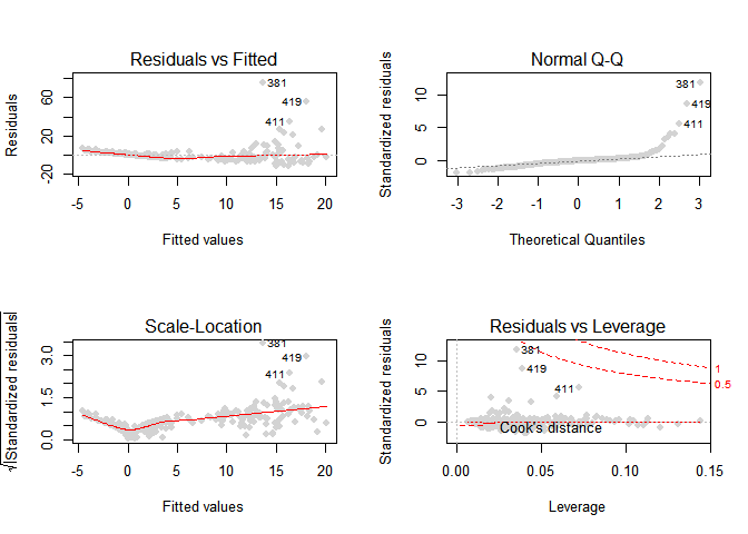
잔차의 분산이 증가하는 추세로 판단되어 이를 해결하기 위해 종속변수의 Concave 함수 변환을 고려하였다.
Log Transformation
featurePlot(x=Boston[,preds],y=log(Boston$crim),pch=20,cex=1.2)
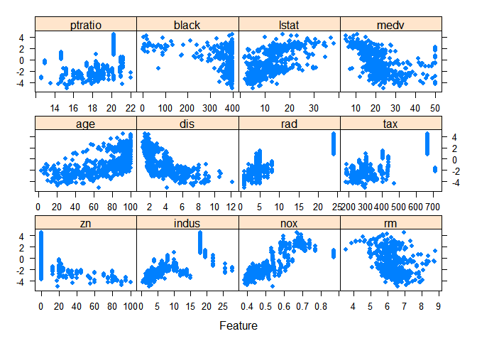
변환 결과 눈에 띄는 독립, 종속 변수간 선형성이 확보되었다.
성능 측면에서도, 모든 독립변수를 사용하고 종속 변수 crim 만 log 변환하여 다중선형회귀를 적합한 결과 모형의 R-Squared 는 크게 증가하였지만 RMSE는 조금 증가하는 모습을 보였다.
## multiple linear regression model 0
lm.alllog=lm(log(crim)~.,data=train)
##
cat('Adjusted R-Squared :',summary(lm.alllog)$adj.r.squared,'\n')
## Adjusted R-Squared : 0.8729427
train_y=predict(lm.alllog,newdata=train)
test_y=predict(lm.alllog,newdata=test)
##
cat('Training RMSE : ',rmse(exp(train_y),train$crim),'\n')
## Training RMSE : 6.61039
cat('Test RMSE : ',rmse(exp(test_y),test$crim),'\n')
## Test RMSE : 6.60867
또한 앞서 확인했던 Collinearity 문제를 살펴보자.
corrplot(cor(Boston[,preds]),method='square')

변수 간의 다중공선성이 존재한다. 이를 vif 함수를 이용해 찾아보겠다.
library(car)
## Loading required package: carData
vif(lm.alllog)
##       zn    indus     chas      nox       rm      age      dis      rad
## 2.308185 3.729722 1.087154 4.470080 2.242700 3.121104 4.132339 7.443892
##      tax  ptratio    black    lstat     medv
## 9.125379 1.991624 1.337849 3.549093 3.671576
독립변수의 분산팽창계수값이 출력되었다. 값을 보니 10을 넘는 독립변수는 존재하지 않는다.
Additional Variable Transformations
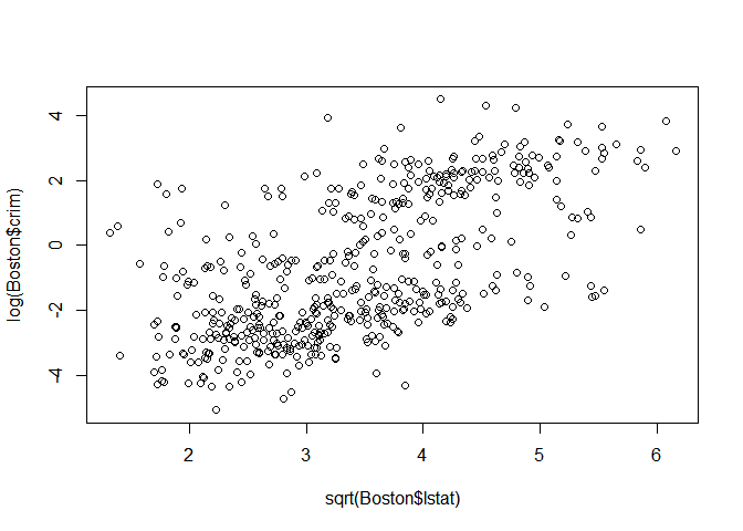
Sqrt(LSTAT)
plot(sqrt(Boston$lstat),log(Boston$crim))
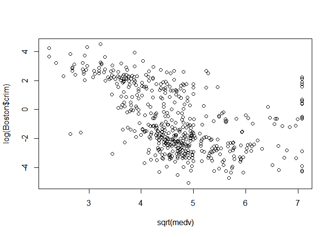
Sqrt(MEDV)
plot(sqrt(medv),log(Boston$crim))
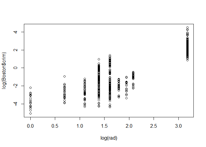
Log(RAD)
plot(log(rad),log(Boston$crim))
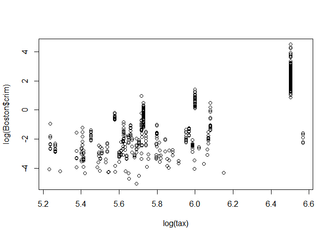
Log(TAX)
plot(log(tax),log(Boston$crim))
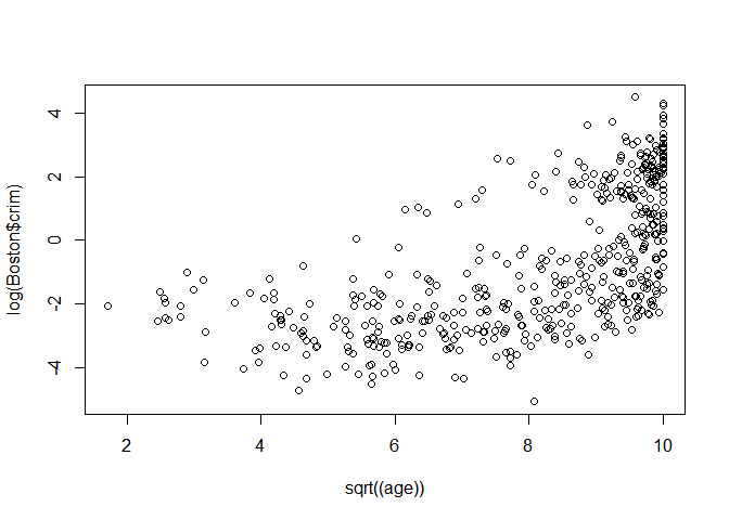
Sqrt(AGE)
plot(sqrt((age)),log(Boston$crim))
Log(DIS)
plot(log(dis),log(Boston$crim))

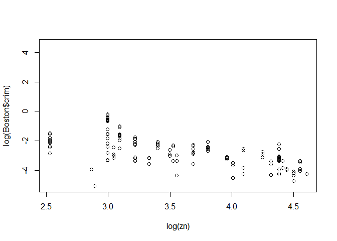
Log(ZN)
plot(log(zn),log(Boston$crim))
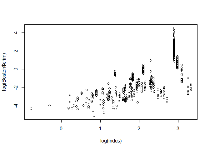
Log(INDUS)
plot(log(indus),log(Boston$crim))
Log(NOX)
plot(log(nox),log(Boston$crim))
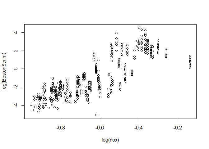
lm.final1=lm(log(crim)~sqrt(lstat)+sqrt(medv)+log(rad)+log(tax)+sqrt(age)+log(dis)+(zn)+log(indus)+log(nox),data=train)

summary(lm.final1)
##
## Call:
## lm(formula = log(crim) ~ sqrt(lstat) + sqrt(medv) + log(rad) +
##     log(tax) + sqrt(age) + log(dis) + (zn) + log(indus) + log(nox),
##     data = train)
##
## Residuals:
##     Min      1Q  Median      3Q     Max
## -2.0719 -0.5195 -0.0594  0.5055  2.2962
##
## Coefficients:
##              Estimate Std. Error t value Pr(>|t|)
## (Intercept) -6.864934   1.495321  -4.591 5.93e-06 ***
## sqrt(lstat)  0.126453   0.082002   1.542   0.1239
## sqrt(medv)  -0.018809   0.079528  -0.237   0.8132
## log(rad)     1.056101   0.082449  12.809  < 2e-16 ***
## log(tax)     0.872048   0.208532   4.182 3.56e-05 ***
## sqrt(age)    0.040039   0.034053   1.176   0.2404
## log(dis)    -0.314417   0.167572  -1.876   0.0613 .
## zn          -0.005383   0.002439  -2.207   0.0279 *
## log(indus)   0.140990   0.093822   1.503   0.1337
## log(nox)     2.570235   0.452253   5.683 2.57e-08 ***
## ---
## Signif. codes:  0 '***' 0.001 '**' 0.01 '*' 0.05 '.' 0.1 ' ' 1
##
## Residual standard error: 0.7894 on 396 degrees of freedom
## Multiple R-squared:  0.8695, Adjusted R-squared:  0.8665
## F-statistic: 293.1 on 9 and 396 DF,  p-value: < 2.2e-16
lm.final2=lm(log(crim)~log(rad)*zn+log(tax)+log(dis)+log(nox),data=train)
summary(lm.final2)
##
## Call:
## lm(formula = log(crim) ~ log(rad) * zn + log(tax) + log(dis) +
##     log(nox), data = train)
##
## Residuals:
##      Min       1Q   Median       3Q      Max
## -1.96582 -0.50396 -0.00454  0.49870  2.24887
##
## Coefficients:
##              Estimate Std. Error t value Pr(>|t|)
## (Intercept) -4.953929   1.161620  -4.265 2.50e-05 ***
## log(rad)     1.231726   0.091695  13.433  < 2e-16 ***
## zn           0.007350   0.004186   1.756 0.079889 .
## log(tax)     0.724318   0.203846   3.553 0.000426 ***
## log(dis)    -0.378470   0.145468  -2.602 0.009620 **
## log(nox)     2.997089   0.421411   7.112 5.33e-12 ***
## log(rad):zn -0.013934   0.003106  -4.487 9.47e-06 ***
## ---
## Signif. codes:  0 '***' 0.001 '**' 0.01 '*' 0.05 '.' 0.1 ' ' 1
##
## Residual standard error: 0.7809 on 399 degrees of freedom
## Multiple R-squared:  0.8713, Adjusted R-squared:  0.8694
## F-statistic: 450.2 on 6 and 399 DF,  p-value: < 2.2e-16
cat('Adjusted R-Squared :',summary(lm.final2)$adj.r.squared,'\n')
## Adjusted R-Squared : 0.8693522
train_y=predict(lm.final2,newdata=train)
test_y=predict(lm.final2,newdata=test)
##
cat('Training RMSE : ',rmse(exp(train_y),train$crim),'\n')
## Training RMSE : 6.954659
cat('Test RMSE : ',rmse(exp(test_y),test$crim),'\n')
## Test RMSE : 6.103154